Getting started tutorial#
The Model Live Diagnostics framework is designed to provide useful and practical Jupyter-based tools for the monitoring and diagnostic analyses of currently running (aka ‘live’) ACCESS climate models on the Australian NCI supercomputer Gadi.
The ACCESS-NRI Model Live Diagnostics package, and the tools that support it, are still a work in progress. We value your feedback, especially in the form of reporting issues/bugs or suggesting ways to improve the framework. To do so, please open an issue here.
What does this package do?#
The primary purpose of the ACCESS-NRI Model Live Diagnostics package is to provide a simple, easy to use and accessible framework for the ACCESS modelling community to check, monitor, visualise and evaluate model behaviour and progress on currently running or ‘live’ ACCESS models on the Australian NCI supercomputer Gadi. In addition to monitoring a live model, the package provides the functionality to load, visualise and compare legacy ACCESS model data with the selected live user model.
This package is currently in active development within the Model Evaluation Team at the Australian Earth System Symulator (ACCESS-NRI) so watch this space for version updates containing new features, model diagnostics tools and visualisation options!
The full docs for MLD can be found here.
0. Install and start and ARE Session#
As described in the homepage of this documentation, you need to clone the MLD repository and start an ARE JupyterLab Session.
1. Set up access#
Now, lets import the med_diagnostics package that has been cloned to an accessbile project location on Gadi
# Import med_diagnostics package
import med_diagnostics

# Import to display tutorial images only
from IPython.display import Image
2. Create live model session#
model_type: str (Type of ACCESS model (e.g. CM2, OM2)).
model_path: str (Path to model output directory/files on Gadi.)
Optional:#
period: int/float/str (Period in minutes for background scheduler to monitor model_path for new data. If period=None, defaults to 60).
timezone: str (Timezone required for scheduler in tinfo ‘Region/Location’ format. Default = ‘Australia/Canberra’)
The CreateModelDiagnosticsSession() class instance triggers the following tasks in the background:#
Start the background scheduler to check for data at the nominted period
Start the dask cluster
Retrieve the most up to date nominated model data and build a new ESM datastore. N.B. This is saved as a compressed *.csv in the user’s $HOME directory on Gadi
Creates both the blue ‘status’ and orange ‘catalog’ information boxes.
session = med_diagnostics.session.CreateModelDiagnosticsSession(model_type='CM2',
                                                                model_path='path/to/your/live/model/data/output')
3. Using the interface#
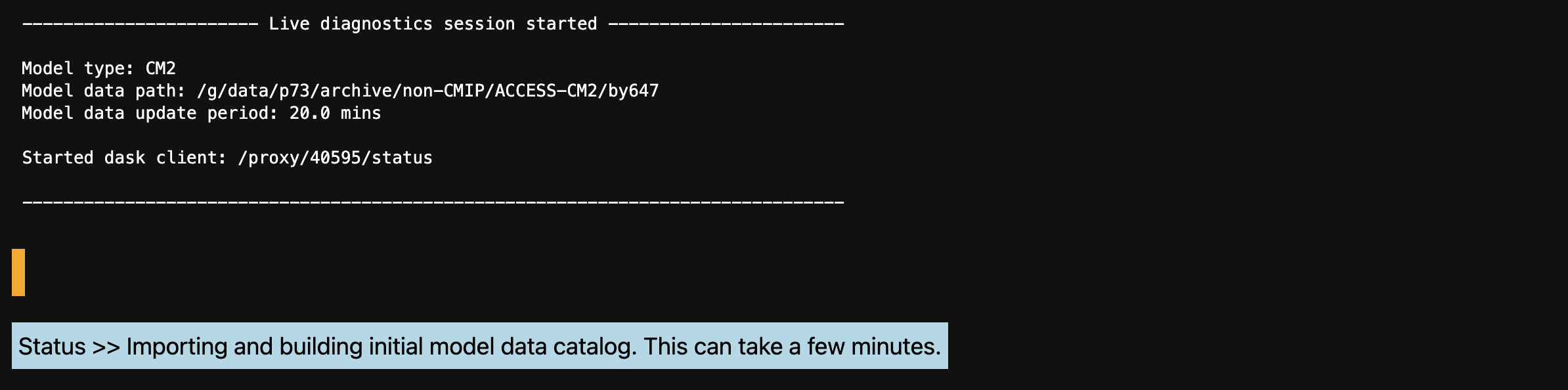
i) Once a session is started, you will see the following sesion summary and blue status message while the new intake catalog is being built from the live model data. Depending on the size of the model data, this can take a number of minutes. The dask cluster address (in this case: /proxy/40595/status) can be used to monitor data retrieval by adding it to the ‘Dask Dashboard URL’ found in the left panel.
ii) Once the live model data catalog has been successfully built, the blue status message will update and the orange status message will report the time and date of the last live model catalog build.
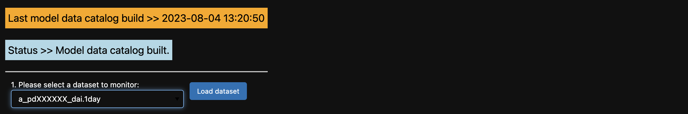
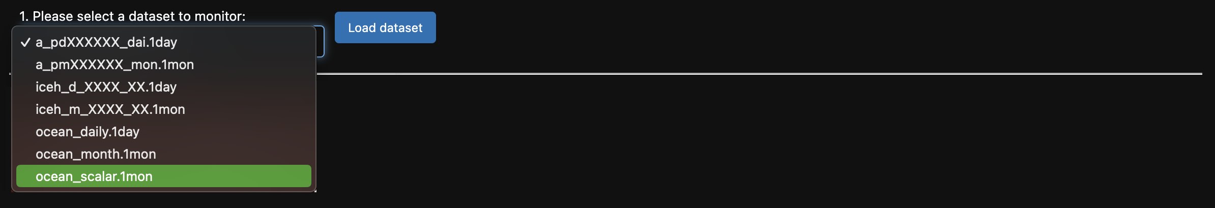
iii) All available datasets from the selected model will be listed in the dropdown. Select the dataset you wish to monitor and click ‘Load dataset’.
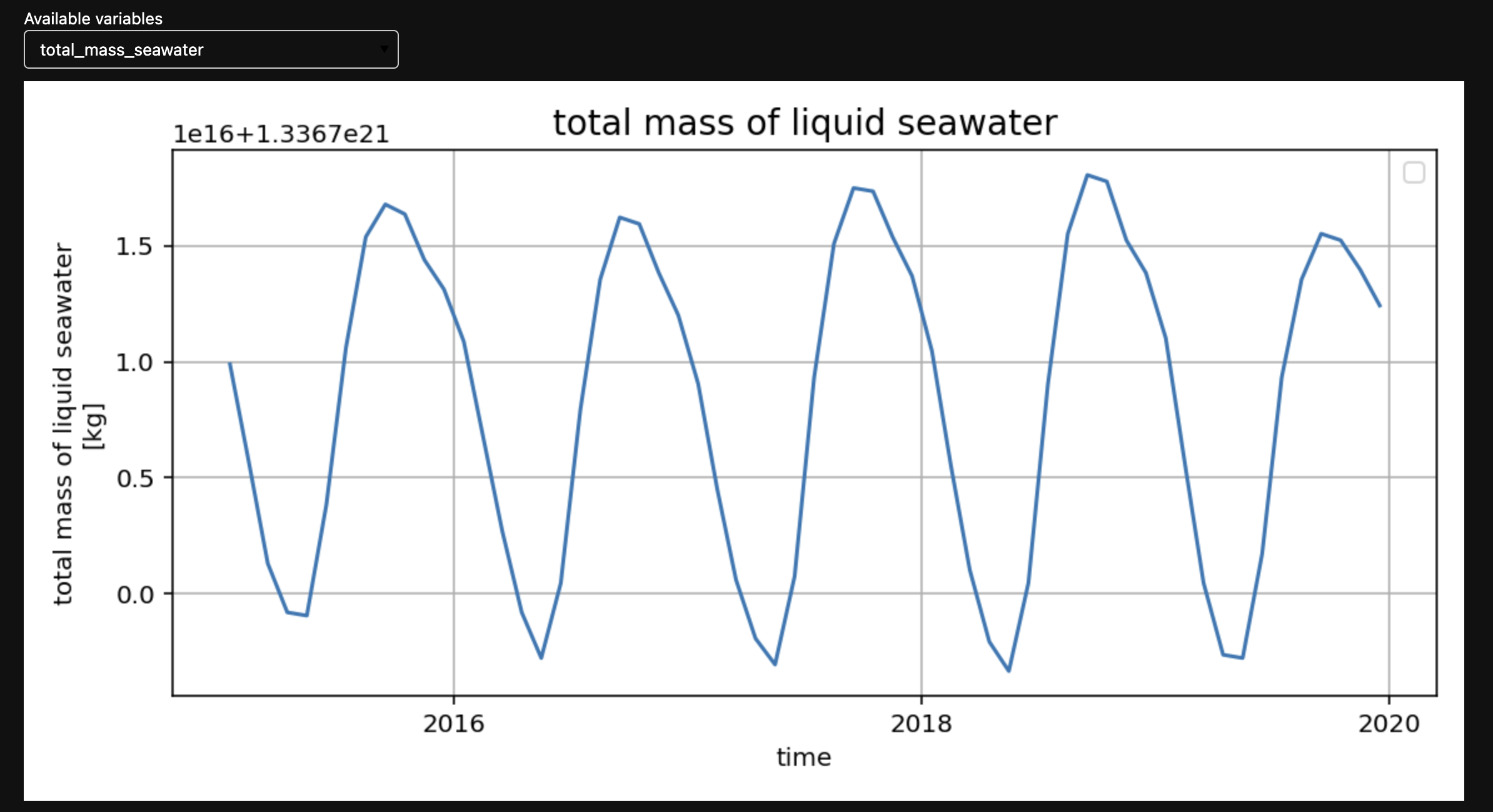
iv) Once loaded, a plot displaying the first data variable in the list will appear. Use the dropdown list to select and plot any available model variables.
Optional:#
The live model data can be compared with any alternative/legacy ACCESS models of the same type (i.e. CM2, OM2 etc) found within the ACCESS-NRI Intake Catalog.
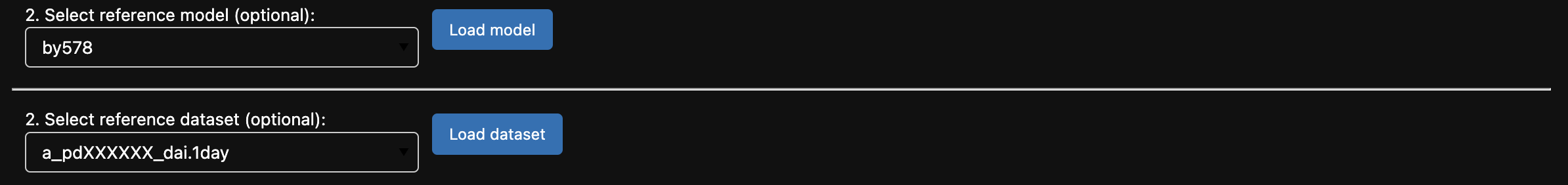
v) The reference model dropdown menu is pre-filled with all available models of the same type from the ACCESS-NRI Intake Catalog (in this example the list contains all models of type ‘CM2’). Select the reference model of choice and click ‘Load model’.

vi) If an optional reference model has been selected, a reference dataset dropdown menu will appear displaying all available datasets from the selected reference model. Select the dataset you wish to monitor and click ‘Load dataset’.
vii) Once loaded, a plot displaying the first data variable in the list will appear. Use the dropdown list to select and plot any available reference model variables. N.B. Unlike the live model plot above, if multiple flavours of a particular model exist (e.g. b7578a, by578b etc), all variants will be displayed.

4. End live model session#
The safest way to end the current live session is to use the session.end_session() function which ends both the dask and background scheduler processes.
session.end_session()